White-Box Adversarial Example

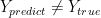
One possible way to evade V2Ray deep neural network traffic classifier is to encode the network traffic with adversarial noise.

To simplify the problem, let’s have the following assumptions:

1. We own the classifier model.
2. We are oracles. Thus, we know the first 16th non-empty TCP payload traffic ahead.
3. We can apply adversarial noise without any restrictions.

You can argue that none of the assumptions are valid in our case. But we may figure out how to remove our assumption one-by-one later. First, I want to do a PoC on the adversarial example idea by trial and error.

Nobody proposed an adversarial example to attack the machine learning model until a deep neural network can reach unprecedented high accuracy in image classification. The math behind generating adversarial examples is straightforward.

Let say we have a binary network traffic classifier

where input X is the network traffic and scalar is the probability of V2Ray network traffic.

Because we have a powerful classifier like almighty God (it has been proven).

{V2Ray traffic},

{non-V2Ray traffic},

Our goal is to find adversarial noise , such that

Because this is a binary classifier. The targeted attack is the same as the untargeted attack. If this were multi-class classifier, you could perform targeted attack by specifying or perform untargeted attack by specifying .

In DNN, is usually a non-linear function. It is not trivial to compute by solving the function directly. Therefore, it is a good topic to write your Ph.D. dissertation on this.

The usual approach is to use the gradient to approximate the adversarial noise. I have tried Fast Gradient Sign Method (FGSM), DeepFool and Jacobian-based Saliency Map (JSMA). I found FGSM is the most effective one for the binary classifier. I will explain the math behind it below.

When train the DNN classifier, we also define loss function where X is the input, is network parameters and is the supervised learning labels. The goal of training is to minimize the loss function by adjusting (learning) the network parameters . We use mini-batch gradient descent to do optimization.

Now we do the opposite thing for generating adversarial examples. We already have a trained model. Thus, we have a set of fixed values for the network parameters . Instead of the supervised learning labels , we use our targeted label . In our V2Ray classifier’s context, the targeted label is 0 — the probability of V2Ray traffic for any true V2Ray traffic is 0.

We want to minimize the loss function by finding input X. So we have the following optimization problem to solve:

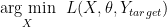
We use a similar optimization approach — gradient descent but on the input rather than the network parameters :

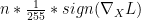
We want the adversarial noise as minimal as possible. FGSM suggests that the size of the gradient doesn’t matter for the adversarial example generation. But the direction of the gradient does matter. Thus, get the direction of the gradient by using sign function and then apply a universal scalar value.

How can we come up a universal scalar value? It depends on your input . For the packet data, each byte is in [0, 255] value range. After normalization by mapping the integer value into [0, 1] real value, its smallest discrete value change is . Therefore, a possible scalar value is , where n is an integer that we need to figure out by inference from the trained model until the prediction turns into our desirable label. In summary, we have the formula below:

adversarial noise =

In practice, I found FGSM approach is better than DeepFool and JSMA.

• Both DeepFool and JSMA need to compute forward gradient on w.r.t . But the activation function of the output layer in the binary classifier is sigmoid function. The function is saturated at both ends. Thus, it suffers the vanishing gradient problem. I got zeros most of the time when computing the forward gradient. But FGSM doesn’t have such a problem. Because it computes forward gradient on the loss function.
• FGSM requires less computation than DeepFool and JSMA. FGSM only need to compute the gradient once. Then loop model inference to get the proper scalar. The other two requires multiple gradient calculation in the loop.

Now let me show you show code and image. I published the Python notebook in my Github. You can replicate my experiment if you collect network traffic by yourself.

I plotted the adversarial noise as an image for input batch = 32. The color red is 1, green is -1, blue is 0, black is the borderline drawn between examples.

I found that:

1. There is always a blue line in the last packet in each example. It seems that the 16th packet is irrelevant.
2. From my eyeballs, there are common patterns in the adversarial noise. This suggests that a universal adversarial noise that applies to all input may exist.

So far so good. In theory, we can defeat the DNN classifier by adding adversarial noises. The next step is to remove the assumptions one-by-one so that make it possible in our real-world application.